This is a little project I did while learning R where I compared Aaron Judge’s 2022 season home run total to that of Roger Maris in 1961 and Barry Bonds in 2001. I started by importing all the data from https://baseball-reference.com. The data looked something like this:

judge = read_html("https://www.baseball-reference.com/players/gl.fcgi?id=judgeaa01&t=b&year=2022") %>%
  html_nodes("table") %>%
  html_table()
judge = data.frame(judge[[5]])

maris = read_html("https://www.baseball-reference.com/players/gl.fcgi?id=marisro01&t=b&year=1961") %>%
  html_nodes("table") %>%
  html_table()
maris = data.frame(maris[[5]])

bonds = read_html("https://www.baseball-reference.com/players/gl.fcgi?id=bondsba01&t=b&year=2001") %>%
  html_nodes("table") %>%
  html_table()
bonds = data.frame(bonds[[5]])

head(judge)

  Rk Gcar Gtm       Date Team Var.6 Opp      Result  Inngs PA AB R H X2B X3B HR
1  1  573   1 2022-04-08  NYY       BOS W, 6-5 (11) CG(11)  5  5 1 2   1   0  0
2  2  574   2 2022-04-09  NYY       BOS      W, 4-2     CG  4  3 1 0   0   0  0
3  3  575   3 2022-04-10  NYY       BOS      L, 3-4     CG  5  5 0 2   0   0  0
4  4  576   4 2022-04-11  NYY       TOR      L, 0-3     CG  4  3 0 0   0   0  0
5  5  577   5 2022-04-12  NYY       TOR      W, 4-0     CG  4  4 0 1   1   0  0
6  6  578   6 2022-04-13  NYY       TOR      L, 4-6     CG  5  4 1 2   0   0  1
  RBI SB CS BB SO   BA  OBP  SLG   OPS TB GIDP HBP SH SF ROE IBB BAbip  aLI
1   0  0  0  0  1 .400 .400 .600 1.000  3    0   0  0  0   0   0  .500 1.20
2   0  0  0  1  0 .250 .333 .375  .708  0    0   0  0  0   0   0  .000 1.01
3   0  1  0  0  2 .308 .357 .385  .742  2    1   0  0  0   0   0  .667 1.86
4   0  0  0  1  2 .250 .333 .313  .646  0    0   0  0  0   0   0  .000 1.27
5   0  0  0  0  0 .250 .318 .350  .668  2    0   0  0  0   0   0  .250 0.56
6   1  0  0  1  1 .292 .370 .500  .870  5    0   0  0  0   0   0  .500 1.33
     WPA acLI   cWPA  RE24 DFS.DK. DFS.FD. BOP   Pos
1 -0.002 1.17  0.00% -0.19   10.00   12.20   2    RF
2  0.006 1.02  0.00% -0.13    4.00    6.20   2 CF RF
3 -0.043 1.89 -0.03%  0.41   11.00   12.00   3    RF
4 -0.039 1.31 -0.02% -0.28    2.00    3.00   3    RF
5 -0.037 0.55 -0.02%  0.49    5.00    6.00   2 CF RF
6  0.119 1.36  0.07%  0.94   19.00   24.70   2    RF

I obviously didn’t need all of these columns, and some of them are the wrong data type, so the next thing I did remove all the columns I didn’t need, and convert the ones I did need from character types to what I wanted. Now it looked like this:

# change "Date" column values fram characters to "Date" type
judge["Date"] <- as.Date(judge$Date)
maris["Date"] <- as.Date(maris$Date)
bonds["Date"] <- as.Date(bonds$Date)

# change "HR" column values from characters to numeric
judge["HR"] <- suppressWarnings(as.numeric(judge$HR))
maris["HR"] <- suppressWarnings(as.numeric(maris$HR))
bonds["HR"] <- suppressWarnings(as.numeric(bonds$HR))

# change "Gtm" column values from characters to numeric (and remove games they missed)
judge["Gtm"] <- as.numeric(str_first_number(judge$Gtm))
maris["Gtm"] <- as.numeric(str_first_number(maris$Gtm))
bonds["Gtm"] <- as.numeric(str_first_number(bonds$Gtm))

# select only the columns I want (and remove null values)
judge = na.omit(select(judge, Gtm, Date, HR))
maris = na.omit(select(maris, Gtm, Date, HR))
bonds = na.omit(select(bonds, Gtm, Date, HR))

head(judge)

  Gtm       Date HR
1   1 2022-04-08  0
2   2 2022-04-09  0
3   3 2022-04-10  0
4   4 2022-04-11  0
5   5 2022-04-12  0
6   6 2022-04-13  1

This looks a lot better, but it’s still not quite what I wanted. For one I wanted cumulative home run totals, not the per-game numbers. I also wanted to combine double-headers so that the tables were only organized by date, as well as remove the games in which they didn’t hit home runs in order to clean up the data.

# add column with cumulative homer total
cumHRs = cumsum(judge["HR"])
colnames(cumHRs) = "cumHRs"
judge = cbind(judge, cumHRs)

cumHRs = cumsum(maris["HR"])
colnames(cumHRs) = "cumHRs"
maris = cbind(maris, cumHRs)

cumHRs = cumsum(bonds["HR"])
colnames(cumHRs) = "cumHRs"
bonds = cbind(bonds, cumHRs)

# remove games in which they don't homer
judge = judge[which(judge$HR > 0 | judge$cumHRs == 0), ]
maris = maris[which(maris$HR > 0 | maris$cumHRs == 0), ]
bonds = bonds[which(bonds$HR > 0 | bonds$cumHRs == 0), ]

tail(judge)

    Gtm       Date HR cumHRs
137 136 2022-09-07  1     55
143 142 2022-09-13  2     57
147 146 2022-09-18  2     59
148 147 2022-09-20  1     60
156 155 2022-09-28  1     61
163 161 2022-10-04  1     62

Finally, I could combine all three players’ tables and create an animated graph showing the home run race over time. Here is the final product:

# add column with players' names (for graphing purposes)
judge = cbind(Player = "Judge", judge)
maris = cbind(Player = "Maris", maris)
bonds = cbind(Player = "Bonds", bonds)

# combine the player data
allGames = rbind(judge, maris, bonds)

# create animated graph
graph <- ggplot(allGames, aes(x=Gtm, y=cumHRs, group=Player, color=Player)) +
  geom_line() +
  geom_point() +
  ggtitle("MLB Home Run Race") +
  theme_ipsum() +
  ylab("Home Runs") +
  xlab("Game") +
  transition_reveal(Gtm) +
  theme(aspect.ratio=3/4)

animate(graph, fps = 7, end_pause = 10)

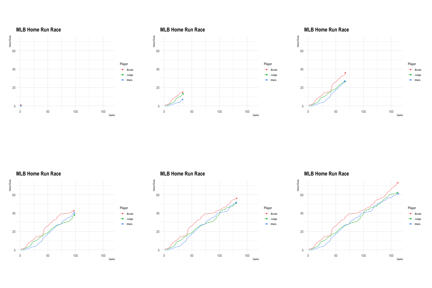
The cool thing about this program is that even though I wrote this while the season was ongoing, it gathers the data from the web so that it’s always up to date. Also because of this, I can easily edit the code if I decide to compare different players in different seasons.